Logistic Regression in SPSS

Blog, Thesis writing

Logistic Regression in SPSS

Logistic Regression is a supervised learning technique, which is used to understand the relationship between a dependent variable and one or more independent variables. Logistic regression is conducted by estimating the probabilities and by using the logistic regression equation.

Assumptions

1. Logistic regression requires the dependent variable to be binary, i.e., 0 and 1.

2. Logistic regression requires the observations to be independent of each other.

3. No Multicollinearity is assumed among the independent variables.

4. Linearity of independent variables and log odds is assumed.

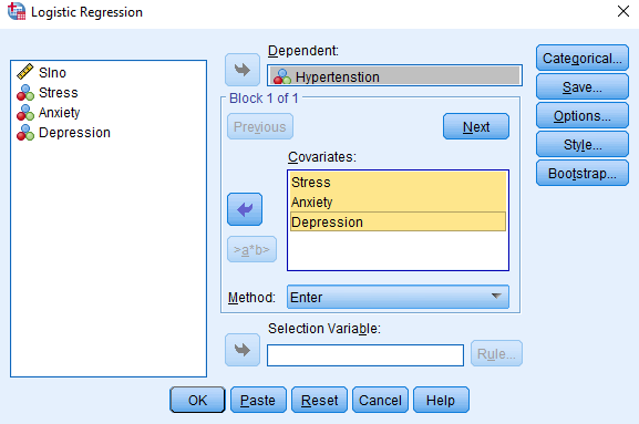
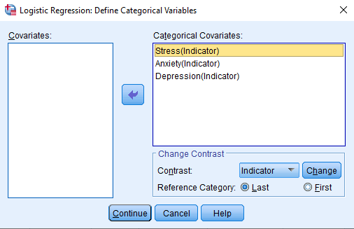
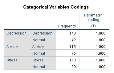
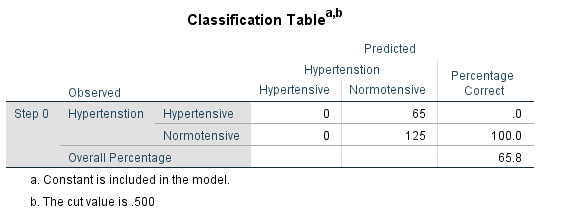
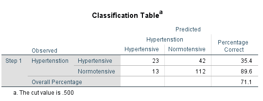
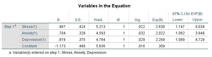
Here, we have taken Hypertension as a dependent variable and we have considered Stress, Anxiety and Depression as the independent variables. 

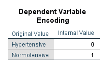
In the dependent variable (Hypertension), we labelled 0 as ‘Hypertensive’ and 1 as ‘Normotensive’. In the independent variables (Stress, Anxiety and Depression), we labelled 0 as ‘Stress’ and 1 as ‘Normal’, 0 as ‘Anxiety’ and 1 as ‘Normal’, and 0 as ‘Depression’ and 1 as ‘Normal’.

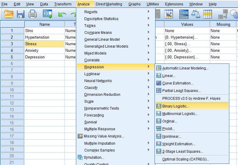
In SPSS, Logistic Regression is found in Analyze > Regression > Binary Logistic Regression

Then, we will get Logistic Regression dialog box.

We have to add the dependent variable (Hypertension) in the ‘Dependent’ box and add the independent variables (Stress, Anxiety, and Depression) in the ‘Covariates’ box.

In the Categorical dialog box, add the categorical variables (Stress, Anxiety, and Depression) into the ‘Categorical Covariates’ box from the ‘Covariates’ box.

In the ‘Change Contrast’ group, change the reference category and then click on ‘Change’ button.

Here, people with anxiety are compared with normal people. Here, normal people are acting as a reference category and thus ‘Last’ is chosen. Then, click on ‘Continue’.

In the ‘Options’ dialog box, add ‘CI for exp(B)’ in the ‘Statistics and Plots’ group and add ‘At last step’ in the ‘Display’ group.

Click on ‘Continue’ and ‘Ok’.

Output of Logistic Regression

First, we will get the ‘Case Processing Summary’ table, and then the ‘Dependent Variable Encoding’ and ‘Categorical Variable Codings’ tables.

These tables give information about the cases that were included and excluded from the analysis, coding of the dependent variable, and coding of the independent categorical variables.

Next, we will get the ‘Classification Table’, ‘Variables in the Equation’ and ‘Variables not in the Equation’ tables for the beginning block. These tables give the output of a null model that has no predictors and has just the intercept.

Then, we will get the tables for the model with predictors.

 First, we will get the ‘Omnibus Tests of Model Coefficients’.

This table gives the Chi Square statistic and its significance level. Here, statistics for ‘Step’, ‘Model’ and ‘Block’ are the same because we have not used stepwise logistic regression or blocking.

The model was statistically significant when compared to the null model (Chi Square = 18.866, P value = 0.000).

Then, we will get the ‘Model Summary’ table.

‘Model Summary’ table contains the ‘Cox & Snell R Square’ and ‘Nagelkerke R Square’ values, which are used for calculating the explained variation. Nagelkerke’s R square is normally used and it is a version of the Cox & Snell R square that adjusts the scale of the statistic to cover the full range from 0 to 1. In this case, we can say that 13.1% change in the dependent variable can be accounted by the predictor variables in the model.

After this, we will get the ‘Classification Table’.

‘The cut value is .500’ – This means that if the probability of a case being classified into the ‘Hypertensive’ category is greater than .500, then that particular case is classified as the ‘Hypertensive’ category. Otherwise, the case is classified as the ‘Normotensive’ category.

When we add the independent variables, the model classifies 71.1% of cases correctly (Overall Percentage = 71.1). This is also called as percentage accuracy in classification.

The model predicted 35.4% of participants with hypertension as hypertensive and it predicted 89.6% of participants without hypertension as normotensive.

The ‘Variables in the Equation’ table shows the contribution of each independent variable to the model and its statistical significance.

The Wald test is used to determine the statistical significance of each of the independent variables. We can see from the results that stress (p = 0.022), anxiety (p = 0.032) and depression (p = 0.029) have significant impact on hypertension. By looking at ‘Exp(B)’, the odds of having hypertension are 2.630 times greater for those who have stress when compared to normal people.

Data: Logistic_Regression_Data.sav

“Rehoboth Academic Services” is a premium institute supporting PhD & Master’s Thesis since 2013. We offer editing, proofreading, paper preparation, statistical analysis,  formatting and plagiarism checking services. We have helped more than 10000+ research scholars in most of the subjects and universities across the globe in the last eleven years. We also conduct workshops on Art of Thesis Writing, Academic Integrity, Research Paper writing, Systematic Review writing, Increasing citation score, SPSS Foundation & Advanced, Jamovi, JASP, SmartPLS and SEM workshops. If you need our assistance please call + 91 9731988227, +91 9741871657.

Are you interested to attend our Workshops?

Click here to see our future workshop schedule…

Leave a Reply

Your email address will not be published.